Introduction
I previously worked on designing some problem sets for a PhD class. One of the assignments dealt with a simple classification problem using data that I took from a kaggle challenge trying to predict fraudulent credit card transactions. The goal of the problem is to predict the probability that a specific credit card transaction is fraudulent. One unforeseen issue with the data was that the unconditional probability that a single credit card transaction is fraudulent is very small. This type of data is known as rare events data, and is common in many areas such as disease detection, conflict prediction and, of course, fraud detection.
This note compares two common techniques to improve classification with rare events data. The basic idea behind these techniques is to increase the discriminative power of a classification algorithm by over-fitting on the rare events. One technique attempts to use sampling weights in the likelihood function itself, whereas, the other is a type of case-control design where we over-sample from the rare class. Which is preferrable depends on both predictive performance, as well as, computational complexity. In this example, we will be “fixing” computational complexity by comparing predictive performance across logistic regression models estimated using MLE. The goal of this exercise is to slowly build up better re-sampling techniques, which will allow us to incorporate matching estimator style control-treatment samples.
An additional motivation for this note is that looking under the hood of common ML libraries can be difficult. Given that many of methods are wrappers of C Libraries, tracking down exact implementation can be tedious. One hope of this exercise is to show how using sample_weights in the sklearn library compares to using a stratified sampling procedure I create.
All of the code and a hyperlink to the data are available on my github.
The Problem
To motivate the problem, let’s simply compare our standard likelihood when our data is Bernoulli distributed with a sample weighted likelihood. Assume $Y_{i} \vert X_{i}$ is Bernoulli distributed, with the probablity of $Y_{i}=1$, or $\pi_{i}$, parameterized by the linear function $\betaX_{i}$. Our standard log-likelihood is simply:
\begin{equation} \mathcal{L}(\beta \vert Y, X) = \sum_{Y_{i}==1} ln(\pi_{i}) + \sum_{Y_{i}==0} ln(1-\pi_{i}) \end{equation}
Weighted Maximum Likelihood
A weighted likelihood approach simply attempts to re-weight our data to account for imbalance across classes. We need a little bit of notation, we define:
In our Bernoulli case, there are only two classes, so c only takes two values, $c=0$ or $c=1$. Thus, the weighted log likelihood is simply:
\begin{equation} \mathcal{L}(\beta \vert Y,X,\omega) = \sum_{Y_{i}==1} \omega_{1} ln(\pi_{i}) + \sum_{Y_{i}==0} \omega_{0} ln(1-\pi_{i}) \end{equation}
Stratified Sampling
Instead of incorporating weights directly into the likelihood, we can instead re-balance our data using a re-sampling procedure. We then estimated the standard MLE in (1) on this sample. The approach this note focuses on is a form of stratified sampling. The procedure is as follows:
- Choose a class of data with probability $\omega_{c}$
- Within the choosen class, draw observations with equal likelihood with replacement
Because I am estimating using MLE in both approaches, these techniques are similar in computational complexity. However, as may be clear, the second technique is indifferent to the model you are estimating. This same procedure can be used for SVMs, Neural Networks and more complex models. Furthermore, it is flexible and additional stages of sampling or decision rules for inclusion in the sample can be changed. My next note will focus on an extension of this stratified procedure that attempts to create matched samples based on “closeness” of observations across the classes.
Another thing to note is a peculiarity about sklearn, the library has a StratifiedKFold method in the model_selection library. However, this method creates folds which preserve the balance between the classes. For example, if class 0 has 10 observations and class 1 has 90 observations, the splits will keep the proportion of 0 to 1 the same, i.e. there will always be 1 observation from class 0 to 9 observations from class 1. This procedure would be the limit of the above procedure if you set $\omega_{c} = \mbox{Proportion in Class c}$ and re-ran the procedure an “infinite” number of times.
Quick Summary
To summarize, this exercise will compare predictive performance using two seperate ways to re-weight our data. Given some pre-chosen weights, $(\omega_{0},\omega_{1})$:
- Weighted Maximum Likelihood : minimize weighted likelihood (2)
- Stratified Random Sampling : stratify random sample then minimize standard likelihood (1)
Data Analysis
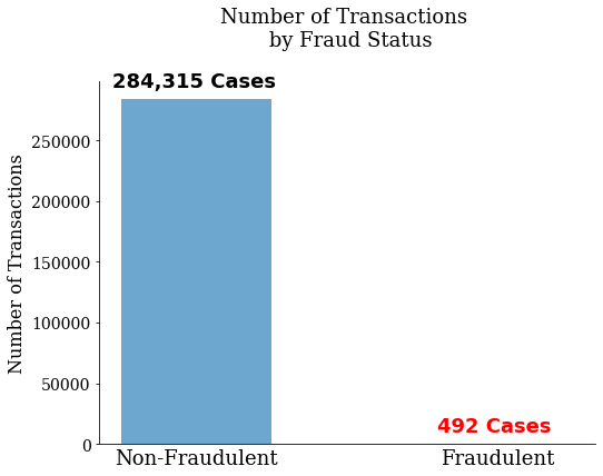
We read in our data and split the dependent and independent variables from one another. Here the independent variable is defined as “Class”. We can see in the graph below that there are only 492 transactions that are fraudulent out of 284,807 total transactions.
import pandas as pd
import numpy as np
import matplotlib.pyplot as plt

# ~ User defined functions ~ #
from user_defined_function import make_frequency_plot
from user_defined_function import make_scores_plot

# ~ Read in our data ~ #
path_to_data="path/to/data"
df=pd.read_csv(path_to_data)

# ~ Split data into dependent and indepent variables ~ #
df=df[[x for x in df.columns if x!='Time']]
iv=df['Class']
dv=df[[x for x in df.columns if x!='Class']]

# ~~ Create plot of frequency of classes ~~ #
make_frequency_plot(iv)
Defining our stratified sampling method
I am doing all this in python. While sklearn has a K-Fold class, which produces K-splits of the data, my specific task requires the following sampling procedure:
- Split data into K-folds defined as $k \in {1,..,K}$
- Within a training set in fold $k$, run our stratified sampling procedure
In order to accomplish this, I extend the KFold class creating the oversample_KFold class. This new class requires a sample weight to sample from each class.
from sklearn.model_selection import KFold
import sklearn.model_selection

class oversample_KFold(KFold):
    '''Extends KFold class for binary datasets to allow for
        stratified sampling (or over-sampling) of the positive
        class

       Methods:
           yield_sample (list) : yields train/test indices after stratified
                                 sampling using sample_weight as the probability
                                 of choosing observations from the positive class

    '''

    # ~ Initialize ~ #
    def __init__(self,*args, **kwargs):
        '''Add sample_weights keyword argument to KFold class'''

        self.sample_weight=kwargs.pop('sample_weight')
        super(oversample_KFold, self).__init__(*args, **kwargs)

    # ~ Extend KFold class to allow oversampling ~ #
    def yield_sample(self,df):
        '''Run KFold split, within the training dataset use a stratified sampling and yield
           test and train indices using this sampling procedure.

           Inputs:
             df (dataframe) : data used in model estimation

           Outputs:
             stratified_train_ix, test_ix (tuple) : tuple of training and test indices
                                                    (same as KFold class)

           Note:

            To form the stratified_train_ix we use the following sampling procedure.
            Create a sample of size df.shape[0]. Within each row, we draw a pair of
            random numbers:

            1. Draw Z from a uniform random.
               If Z <= sample_weight : in step (2) sample from negative class (class = 0)
               If Z >  sample_weight : in step (2) sample from positivie class (class = 1)

            2. Draw W from a discrete uniform distribution with size = # observations in
                the class being drawn from.

               For example, if:
                              sample weight=0.5
                              Z = 0.3
                              Number Obs in Class 0 = 10
                              Number Obs in Class 1 = 20
                            then:
                              W is drawn from discrete uniform with size = 10
                               (i.e. each observation has 1/10 probability)

          These pairs (Z,W) create a new set of indices for our test dataset.

        '''
        # ~ Indices for 0 and 1 class ~ #
        class_0_ix=set(df.loc[df['Class']==0].index.values)
        class_1_ix=set(df.loc[df['Class']==1].index.values)
        for split in KFold(n_splits=self.n_splits,random_state=self.random_state).split(df):
            # ~ Get train/test indices ~ #
            train_ix = split[0]
            test_ix = split[1]
            # ~ Split training data into class 0 and 1 training ~ #
            class_0_train = [x for x in train_ix if x in class_0_ix]
            class_1_train = [x for x in train_ix if x in class_1_ix]
            # ~ Draw a random variable to determine which class to sample ~ #
            select_class_draws = np.random.uniform(size=len(train_ix))<=self.sample_weight
            n_class_0 = sum(select_class_draws==0)
            n_class_1 = sum(select_class_draws==1)
            # ~ Within each class, draw a random number to select each index ~ #
            class_0_draws=np.random.randint(low=0,high=len(class_0_train)-1,size=n_class_0)
            class_1_draws=np.random.randint(low=0,high=len(class_1_train)-1,size=n_class_1)
            oversample_train_index = ([class_0_train[x] for x in class_0_draws] +
                                     [class_1_train[x] for x in class_1_draws])
            # ~ Yield indices for train and test data ~ #
            stratified_train_ix=np.array(oversample_train_ix)
            yield stratified_train_ix, test_ix
Model Pipeline
We create a model pipeline that has the following steps:
-
Seperate categorical and numeric variables
-
Standardize (or one hot encode) variables
-
Concatenate columns together
-
Create full pipeline with data transformations and logistic regression model
# ~~~~~~~~~~~~~~~~~~~~~~~~~~~~~~~~~~~~~~~~~~~~~~~~~~~~~~~~~ #
#                  Setup Model Pipeline                     #
# ~~~~~~~~~~~~~~~~~~~~~~~~~~~~~~~~~~~~~~~~~~~~~~~~~~~~~~~~~ #

# ~~~~ Pipeline + Data Transform Libraries ~~~~ #
from sklearn.preprocessing import StandardScaler, OneHotEncoder
from sklearn.impute import SimpleImputer
from sklearn.compose import ColumnTransformer
from sklearn.pipeline import Pipeline
from sklearn.linear_model import LogisticRegression

# (1) : Seperate numeric and categorical variables
# (2) : Create transforms (imputation + standardization) for both types
numeric_bool=((dv.dtypes=='int64') | (dv.dtypes=='float64'))
numeric_features = list(dv.dtypes[numeric_bool].index.values)
numeric_transformer = Pipeline(steps=[
    ('imputer', SimpleImputer(strategy='median')),
    ('scaler', StandardScaler())])

categorical_features = list(dv.dtypes[((dv.dtypes=='object')) ].index.values)
categorical_transformer = Pipeline(steps=[
    ('imputer', SimpleImputer(strategy='constant', fill_value='missing')),
    ('onehot', OneHotEncoder(handle_unknown='ignore'))])

# (3) : Concatenate columns together and apply transformations
preprocessor = ColumnTransformer(
    transformers=[
        ('num', numeric_transformer, numeric_features),
        ('cat', categorical_transformer, categorical_features)])

# (4) : Create pipeline with preprocessing + estimation steps
clf = Pipeline(steps=[('preprocessor', preprocessor),
                      ('classifier', LogisticRegression(solver='lbfgs',max_iter=1000))])
Model Estimation
This is the meat of this exericse. What we will do is estimate both a weighted logistic regression and a standard logistic regression with stratified random sampling. We will then plot three relevant model score metrics: accuracy, recall and precision. What we will see is how bad accuracy is for predictions of rare events. We will then see how the two strategies differ in their recall versus the precision.
# ~~~~~~~~~~~~~~~~~~~~~~~~~~~~~~~~~~~~~~~~~~~~~~~~~~~~~~~~~~~~~ #
# ~ Run logisitic regression using Weighted MLE v. Stratified ~ #
# ~~~~~~~~~~~~~~~~~~~~~~~~~~~~~~~~~~~~~~~~~~~~~~~~~~~~~~~~~~~~~ #

# ~~ Model estimation + selection libraries ~~ #
from sklearn.model_selection import cross_validate, KFold
from sklearn.metrics import accuracy_score, recall_score, average_precision_score, f1_score, make_scorer

# Set up 10 fold cross-validation with specified random seed
seed=1
n_splits=10

# Initialize KFold Object
kfold_obj = KFold(n_splits=n_splits, random_state=seed)

# Lists to hold scores for model runs
accuracy_list=[]
recall_list=[]
average_precision_list=[]
f1_weighted_list=[]

# Loop through weights
weights=np.arange(0,1.05,0.05)
for sample_weight in weights:
    # ~ Model with no weighting ~ #
    if sample_weight==0:
        scores = cross_validate(clf,dv,iv,cv=kfold_obj,
                        scoring={'accuracy':make_scorer(accuracy_score),
                                 'recall':make_scorer(recall_score),
                                 'average_precision_score':make_scorer(average_precision_score)})
        # ~ Calculate different scoring rules ~ #
        mean_accuracy_weighted=np.mean(scores['test_accuracy'])
        mean_recall_weighted=np.mean(scores['test_recall'])
        mean_avg_precision_weighted=np.mean(scores['test_average_precision_score'])
        mean_accuracy_oversample=mean_accuracy_weighted
        mean_recall_oversample=mean_recall_weighted
        mean_avg_precision_oversample=mean_avg_precision_weighted


    # ~ Model with weighting ~ #
    else:
        # ~ Weighted Likelihood ~ #
        weighted_scores = cross_validate(clf,dv,iv,cv=kfold_obj,
                        scoring={'accuracy':make_scorer(accuracy_score),
                                 'recall':make_scorer(recall_score),
                                 'average_precision_score':make_scorer(average_precision_score)},
                       fit_params={'classifier__sample_weight':[[1-sample_weight,sample_weight][x==1] for x in iv]})

        # ~ Calculate different scoring rules ~ #
        mean_accuracy_weighted=np.mean(weighted_scores['test_accuracy'])
        mean_recall_weighted=np.mean(weighted_scores['test_recall'])
        mean_avg_precision_weighted=np.mean(weighted_scores['test_average_precision_score'])


        # ~ Stratified Sample ~ #
        oversample_kfold_obj = oversample_KFold(n_splits=n_splits,random_state=seed,sample_weight=sample_weight)
        oversampling_scores = scores = cross_validate(clf,dv,iv,cv=oversample_kfold_obj,
                                        scoring={'accuracy':make_scorer(accuracy_score),
                                                 'recall':make_scorer(recall_score),
                                                 'average_precision_score':make_scorer(average_precision_score)})

        # ~ Calculate different scoring rules ~ #
        mean_accuracy_oversample=np.mean(oversampling_scores['test_accuracy'])
        mean_recall_oversample=np.mean(oversampling_scores['test_recall'])
        mean_avg_precision_oversample=np.mean(oversampling_scores['test_average_precision_score'])

    # ~~~ Append data to list ~~~ #
    accuracy_list.append((sample_weight,mean_accuracy_weighted,mean_accuracy_oversample))
    recall_list.append((sample_weight,mean_recall_weighted,mean_recall_oversample))
    average_precision_list.append((sample_weight,mean_avg_precision_weighted,mean_avg_precision_oversample))

# ~~~ Form data frame of scores ~~~ #
scoresDF=pd.DataFrame([(x[0],x[1],'precision','wmle') for x in average_precision_list],
                      columns=['weight','score_value','score','estimator'])
scoresDF=scoresDF.append(pd.DataFrame([(x[0],x[2],'precision','stratified') for x in average_precision_list],
                         columns=['weight','score_value','score','estimator']))
scoresDF=scoresDF.append(pd.DataFrame([(x[0],x[1],'recall','wmle') for x in recall_list],
                      columns=['weight','score_value','score','estimator']))
scoresDF=scoresDF.append(pd.DataFrame([(x[0],x[2],'recall','stratified') for x in recall_list],
                         columns=['weight','score_value','score','estimator']))
scoresDF=scoresDF.append(pd.DataFrame([(x[0],x[1],'accuracy','wmle') for x in accuracy_list],
                      columns=['weight','score_value','score','estimator']))
scoresDF=scoresDF.append(pd.DataFrame([(x[0],x[2],'accuracy','stratified') for x in accuracy_list],
                         columns=['weight','score_value','score','estimator']))


# ~ Scores dataframe ~ #
scoresDF=scoresDF.loc[scoresDF['weight']!=1]
scoresDF.head()
| weight | score_value | score | estimator | |
|---|---|---|---|---|
| 0 | 0.00 | 0.486922 | precision | wmle |
| 1 | 0.05 | 0.233179 | precision | wmle |
| 2 | 0.10 | 0.280194 | precision | wmle |
| 3 | 0.15 | 0.310600 | precision | wmle |
| 4 | 0.20 | 0.335632 | precision | wmle |
Model Performance
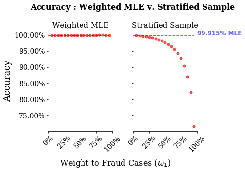
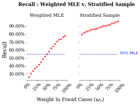
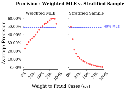
We have three different performance metrics: accuracy, recall and precision. The blue lines in each plot are the metrics value for the standard MLE with no sample weights. The x-axis are the sample weights given to the rare events, or $\omega_{1}$ in our notation above. As you increase this sample weight, you give more weight to rare event options. Note, that I run the models between 0.05 and 0.95, hence why the stratified sample procedure starts above the MLE line. Also, I only ran the re-sampling methods once, thus there is some noise in these estimates. However, given the monotonicity of the lines in the stratified sampling graphs, the sampling error must be minor.
There are two things to note from these graphs. First, accuracy is a bad measure for both of these models. Looking at the stratified sample, even when giving nearly all weight to the stratified sample, the model has an accuracy of around 75%. Second, stratified sampling performs vastly better on recall, and for higher weights vastly worse on precision than weighted MLE.
This dovetails nicely with thinking about the exact loss function you are trying to pin down in this problem. The stakeholders for this sort of algorithm would be a credit card company. For a credit card company, missing an instance of fraud is much worse than calling an instance of non-fraud a fraudulent activity. The company is on the hook for fraudulent charges, so they want to minimize those as much as possible. With that in mind, they may want to detect all the cases of fraud, regardless of the cases of non-fraud. To me, this sounds like recall, the closer to 1 the better. If we just cared about recall, then our stratified sampling model does much better.
However, there is some cost to a credit card company from rejecting too many charges. If you are a customer of a credit card company that denies all your charges, then you would probably get another credit card. In this case, a credit card company probably also care about minimizing false positives. With this in mind, we can look at precision. What we see if for low weights re-sampling does about as good as weighted MLE, but for higher weights it does much worse.
# ~~ Plot all the measurements ~~ #

# ~ Accuracy ~ #
make_scores_plot(scoresDF,'accuracy')

# ~ Recall ~ #
make_scores_plot(scoresDF,'recall')

# ~ Precision ~ #
make_scores_plot(scoresDF,'precision')
Summary
The above exercise shows that model selection metrics are important for your task at hand. When faced with rare events data, accuracy performs poorly, whereas, recall and precision depend on the model at hand. As a follow-up, I hope to show how to improve on the re-sampling procedure. A key place for improvement is the independence in sampling across classes. The current algorithm selects a class, then an observation from that class. However, it may be better to select an observation of interest, say an example of fraud, then select a very similar example of non-fraud to distinguish the differences between them. The underlying idea is that it is easy to spot obvious non-fraud, such as someone purchasing a $4 cup of coffee from their local coffee shop, and these are not the important cases that the algorithm relies upon to train. The idea will be to use the most “informative” points for training.